- LIVE HELP IS

Getting Started Tutorial
-
Open the workbook DMAIC Project Duration. This is an example model of a Six Sigma project with five phases: Define, Measure, Analyze, Improve and Control. We are interested in estimating the total project duration in days. Management requires that the project be completed in 120 days. We will model duration simply as:
Total Duration = Define + Measure + Analyze + Improve + Control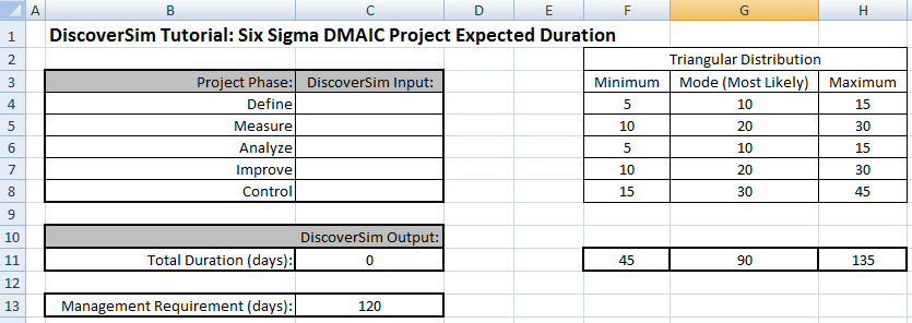
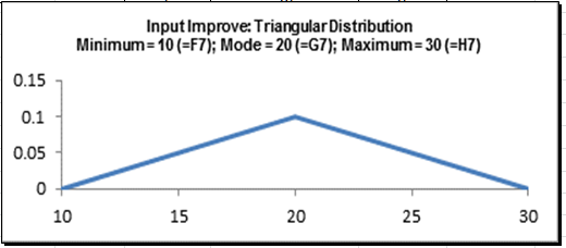
- We will model each phase using a Triangular Distribution, which is popular when data or theory is not available to estimate or identify the distribution type and parameter values. (Another similar distribution that is commonly used for project management is PERT). The Minimum, Mode (Most Likely) and Maximum durations were estimated by the Six Sigma project team based on their experience.
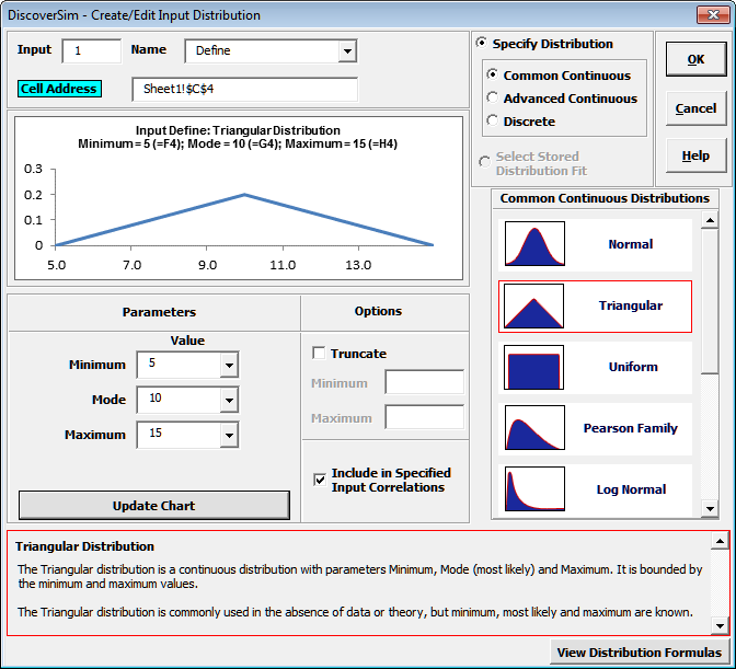
- Click on cell C4 to specify the Input Distribution for Define. Select DiscoverSim >
Input Distribution

- Select Triangular Distribution. A brief description of the Triangular Distribution is given in the dialog.
- Click input Name cell reference
 and specify cell B4 containing the input name “Define”. After specifying a cell reference, the dropdown symbol changes from to
  .
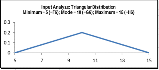
. - Click the Minimum parameter cell reference and specify cell F4 containing the minimum parameter value = 5.
- Click the Mode parameter cell reference and specify cell G4 containing the mode (most likely) parameter value = 10.
- Click the Maximum parameter cell reference and specify cell H4 containing the maximum parameter value = 15.
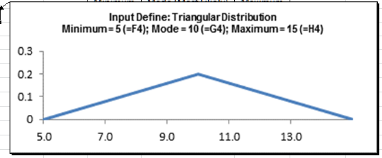
- Click Update Chart to view the triangular distribution as shown:
- Click OK. Hover the cursor on cell C4 to view the DiscoverSim graphical comment showing the distribution and parameter values:
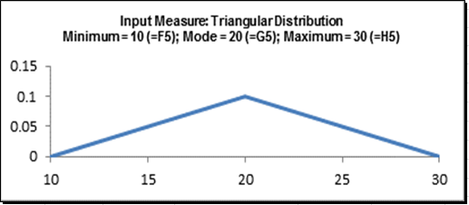
- Click on cell C4. Click the DiscoverSim Copy Cell menu button
 (Do not use Excel’s Copy – it will not work!).
 - Select cells C5:C8. Click the DiscoverSim Paste Cell menu button
 (Do not use Excel’s Paste – it will not work!).
 - Verify that the input comments appear as shown:
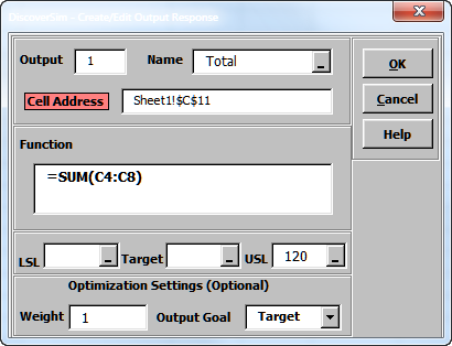
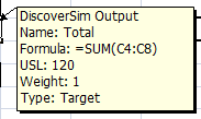
- Click on cell C11. Note that the Excel formula =SUM (C4:C8) has already been entered. Select DiscoverSim > Output Response:
- Enter the output Name as “Total”. Enter the Upper Specification Limit (USL) as 120 (or specify cell reference C13).
- Hover the cursor on cell C11 to view the DiscoverSim Output information.
- Select DiscoverSim > Run Simulation:

- Click Report Options/Sensitivity Analysis. Check Sensitivity Charts and Correlation Coefficients. Select Seed Value and enter “12” as shown, in order to replicate the simulation results given below.
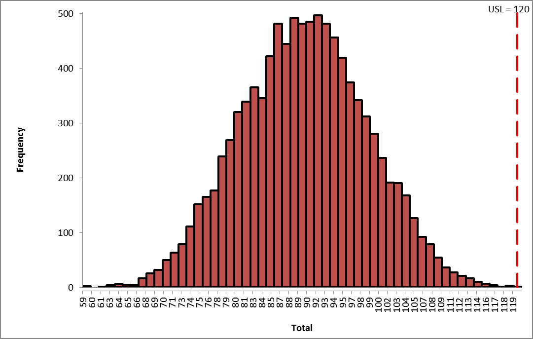
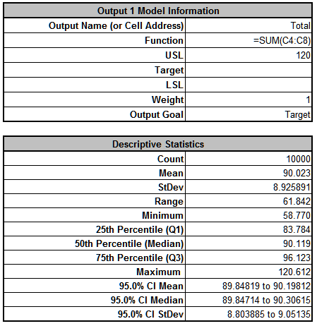
- The DiscoverSim output report shows a histogram, descriptive statistics and process capability indices:
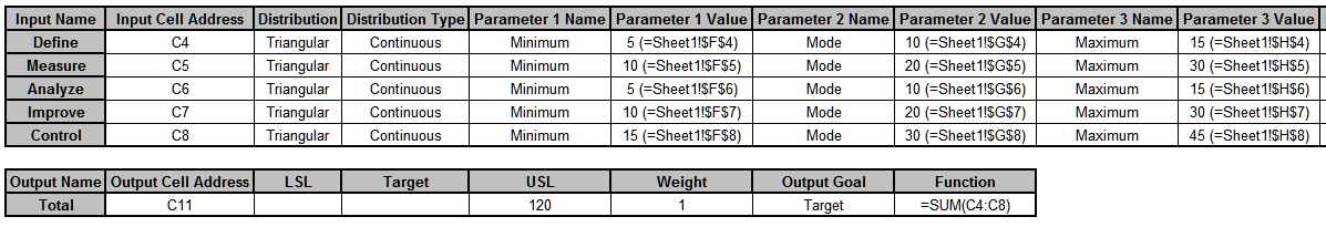
- A summary of the model input distributions, parameters and output response is also given in the simulation report.
- If we needed to improve the performance, the sensitivity charts would guide us where to focus our efforts. Click on the Sensitivity Correlations sheet:
Cell C5
Cell C6
Cell C7
Cell C8

Click OK
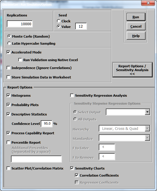
Click Run
 |
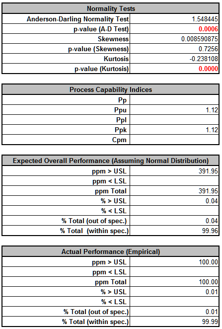 |
From the histogram and capability report we see that the Total Project duration should easily meet the requirement of 120 days, assuming that our model is valid. The likelihood of failure (based on the actual simulation performance) is approximately .01%.
Tip: Use this summary to keep track of simulation runs with modified parameter values.
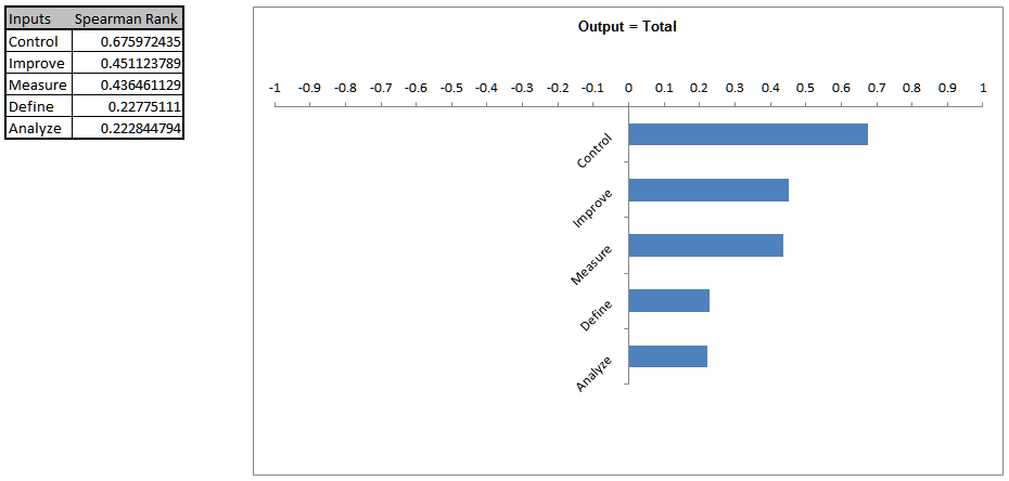
The control phase is the dominant input factor affecting Total Duration, followed by Measure and Improve.
Tip: This Sensitivity Chart uses the Spearman Rank Correlation, and the results may be positive or negative. If you wish to view R-Squared percent contribution to variation, rerun the simulation with Sensitivity Regression Analysis and Sensitivity Charts, Regression Coefficients checked.
The results in this simple example are intuitively obvious from the input values, but keep in mind that a real model will likely be considerably more complex with sensitivity analysis results identifying important factors that one might not have expected.
Define, Measure, Analyze, Improve, Control


Simulate, Optimize,
Realize

Web Demos
Our CTO and Co-Founder, John Noguera, regularly hosts free Web Demos featuring SigmaXL and DiscoverSim
Click here to view some now!
Contact Us
Phone: 1.888.SigmaXL (744.6295)
Support: Support@SigmaXL.com
Sales: Sales@SigmaXL.com
Information: Information@SigmaXL.com


