Multiple Response Optimization

Multiple Response Optimization Example: Robust Cake

Click here for more information about the Multiple Response Optimization dialog and options.

Multiple Response Optimization (MRO) in Advanced Multiple Regression maximizes the Desirability function (with values 0 to 1). For details on the statistical methods, formulas and references, see the Workbook Appendix: Multiple Response Optimization.

We will re-analyze the Robust Cake DOE data from Three Factor Full Factorial Example Using DOE Template and apply Multiple Response Optimization to the Average and Standard Deviation of Taste Score.

1. Open the file DOE Example - Robust Cake.xlsx. This is a Robust Cake Experiment adapted from the Video "Designing Industrial Experiments" by Box, Bisgaard and Fung.
   
   
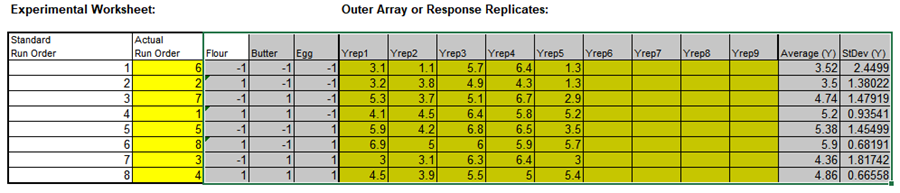
2. The response is Taste Score (on a scale of 1-7 where 1 is "awful" and 7 is "delicious").
   
   
3. The five Outer Array Reps have different Cooking Time and Temperature Conditions. The outer array was a two-factor, full-factorial plus center point, hence 5 replications.
   
   
4. The goal is to Maximize Mean and Minimize StDev of the Taste Score.
   
   
5. The X factors are Flour, Butter, and Egg. Actual low and high settings are not given in the video, so we will use coded -1 and +1 values. We are looking for a combination of Flour, Butter, and Egg that will not only taste good, but consistently taste good over a wide range of Cooking Time and Temperature conditions.
   
   
6. In the Experimental Worksheet, highlight the columns Flour to StDev (Y) (cells D17:Q25) as shown:
   
   
   
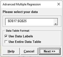
7. Click SigmaXL > Statistical Tools > Advanced Multiple Regression > Fit Multiple Regression Model.
   
   
   
   
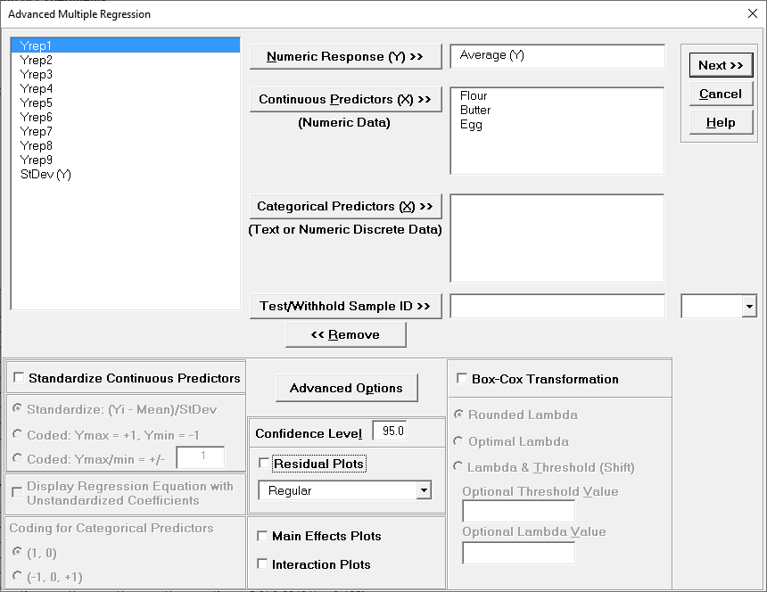
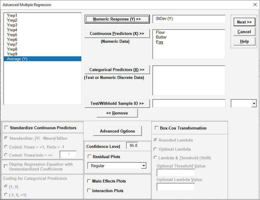
8. Ensure that the data selection is $D$17:$Q$25. Click Next>>. Select Average (Y), click Numeric Response (Y) >>; select Flour, Butter, and Egg; click Continuous Predictors (X)>>. Uncheck Residual Plots, Main Effects Plots and Interaction Plots as we will not be referring to them in this demonstration.
   
   
   
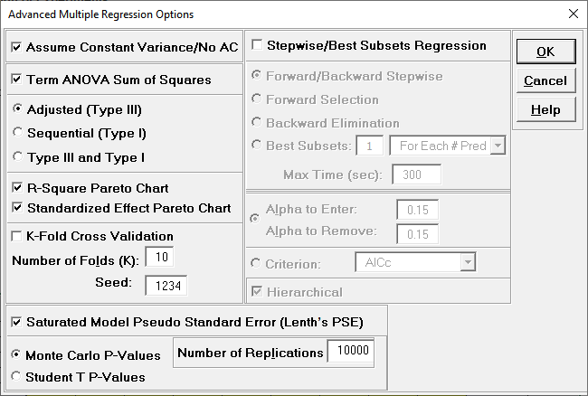
9. Click Advanced Options. We will use the defaults as shown:
   
   
   
10. Click OK. Select ME + 2-Way Interactions. Holding the CTRL key, select Butter, Egg, and Butter*Egg, click Model Terms >.
    
    
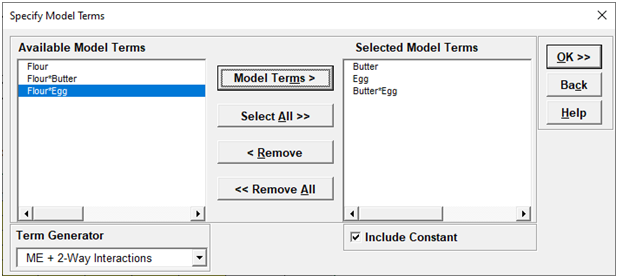
    This matches the final model used in the original analysis of Average (Y).
    
    
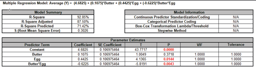
11. Click OK. The Advanced Multiple Regression report for Average (Y) is given:
    
    
    
12. Next, we will create a regression model for StDev (Y). Click Recall Last Dialog (or press F3). Select StDev (Y), click Numeric Response (Y) >>.
    
    
    
13. Click Next >>. Select Flour. Click Model Terms >.
    
    
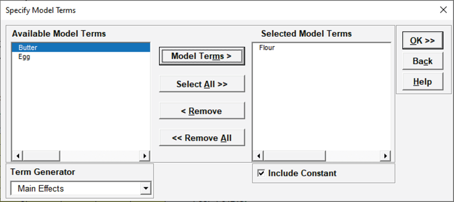
    This matches the final model used in the original analysis of StDev (Y).
    
    
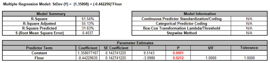
14. Click OK. The Advanced Multiple Regression report for StDev (Y) is given:
    
    
    
15. Now we will simultaneously maximize the Average (Y) and minimize the StDev (Y) using Multiple Response Optimization. Click SigmaXL > Statistical Tools >Advanced Multiple Regression>Multiple Response Optimization.
    
    
16. Select MReg1 - Model Average, click Response 1 >>. Set Goal = Maximize. Select MReg2 - Model StDev, click Response 2 >>. Set Goal = Minimize. We will use the default Lower and Upper values which are derived from the response minimum and maximum, and the default Weight = 1 and Importance = 1 for both responses.
    
    
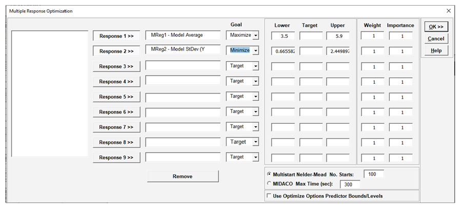
    Note, Target is not required for Goal = Maximize or Minimize.
    
    
17. Click OK >>. The Multiple Response Optimization report is given:
    
    
    
    
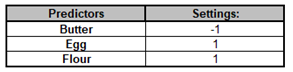
    The Predictor Settings match those used in the original analysis, with Butter = -1, Egg = +1, and Flour = +1. Note, predictor names in this report are sorted alphanumerically.
    
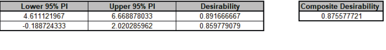
    The Predicted Response values are slightly different than those in the previous analysis because here we are using the refined models, whereas the DOE Template Predicted Output uses the model with all terms included.
    
    MRO maximizes the Composite Desirability score which can be a 0 to 1 value. For more information on the individual and composite desirability scores, see the Appendix: Multiple Response Optimization.
    
    

Multiple Response Optimization Dialog

< Back to top

• Select Responses to use in MRO from the available models in the workbook that have been created using Advanced Multiple Regression.


• If the response, Goal is Target, a Target value must be specified. It must be a value greater than Lower and less than Upper.


• If the response Goal is Maximize or Minimize, Target is not used.


• Lower and Upper limits must always be specified. They can be specification limits or practical limits for maximization/minimization. For maximization, a practical upper limit would be a value beyond which an increase in desirability is not beneficial. For minimization, a practical lower limit is a value below which an increase in desirability is not beneficial. The initial values for Lower and Upper that are given in the dialog are the minimum and maximum response values respectively.


• Importance allows for weighting of the responses according to relative importance. Use a value between 0.1 and 10 (default = 1).


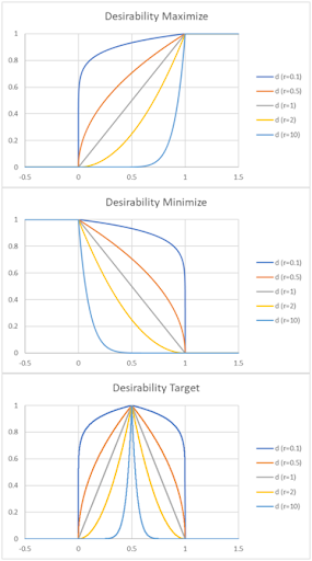
• Weight(r) is a shape factor. For weight = 1 (default), the desirability function increases linearly. For weight < 1, the function is concave, so low priority on hitting the target or goal. For weight > 1, the function is convex, so high priority on hitting the target or goal. Use a value between 0.1 and 10.





• Multistart Nelder-Mead: Nelder-Mead Simplex is derivative free so can accommodate the non-smooth desirability response with both continuous and categorical predictors. It is very fast but gives a local solution. Multistart helps to improve the chances of finding a global solution. If there are a number of equally valid best solutions, the one with the smallest predicted response standard error is chosen.


• MIDACO: Mixed Integer Distributed Ant Colony Optimization (MIDACO) is a global optimizer so would be more suitable for a complex problem with multiple local solutions, but is slower than Nelder-Mead.


• Use Optimize Options Predictor Bounds/Levels: For each specified response model sheet that is used in MRO, continuous predictors can optionally be constrained to a range or specified as integers and categorical predictors can be held to a specified level. If this option is checked, MRO will apply these constraints. If there is a conflict in the constraints across models for a given continuous predictor, the lower bound used in MRO is the maximum of the lower bounds and upper bound is the minimum of the upper bounds. If any of the models flag a continuous predictor as an integer, then it is assumed to be integer continuous for MRO. For categorical levels, if they are inconsistent across models, then MRO will use all levels. In order to constrain MRO to use a specific categorical level, all models must have that same level specified.