This Catapult experiment is adapted from the article "THE CATAPULT PROBLEM: ENHANCED ENGINEERING MODELING USING EXPERIMENTAL DESIGN", by Schubert et. al., Quality Engineering, 4(4), 463-473 (1992).
- Click SigmaXL > Help > Template Examples > Taguchi Examples > L8 Four Factor - Catapult to open the example file. If you wish to start with a blank template and populate the values, click SigmaXL > Design of Experiments > Basic Taguchi DOE Templates > Taguchi L8 (2 Level) > Four Factor (with Aliased Two-Way Interactions).
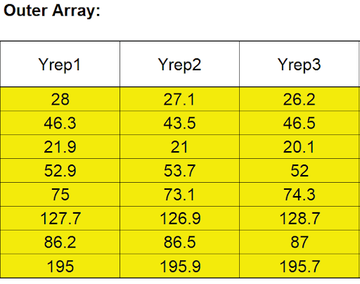
- The response is Distance in Inches with Target = 50".
- The three Outer Array (Yrep1 to Yrep3) values are repeat shots fired.
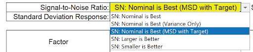
- The goal is to hit a specific target of 50 inches with minimum variation, so we will maximize the Signal-to-Noise Ratio SN: Nominal is Best (MSD with Target), selected from the list as shown:
- Enter the Target value 50 in cell H8 :
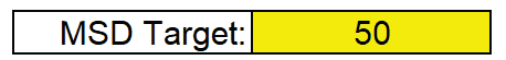
Note: If Target = 0, Nominal is Best (MSD with Target) is equivalent to Smaller Is Better. For use of MSD in SN Ratio, see Ranjit Roy (2010) A Primer on the Taguchi Method, Second Edition, Society of Manufacturing Engineers.
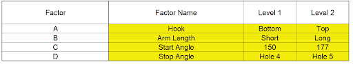
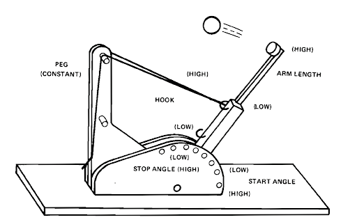
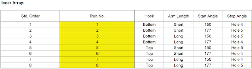
- The Inner Array controllable factors used in this study are: Hook (Bottom/Top), Arm Length (Short/Long), Start Angle (150/177) and Stop Angle (Hole 4/Hole 5).
Note that these are different factors and factor levels than those used earlier in the Full Factorial Catapult experiment (Part C), so the results cannot be compared. In that experiment we used Pull Back Angle, Stop Pin and Pin Height. Here, Pin Height is kept fixed so not included, but Hook position and Arm Length are used. (In typical Catapult designs used in training today, Arm Length is adjusted by varying the Cup position).
- Schubert used a Three Factor 8 Run Resolution IV design. We will use the Taguchi L8 Four Factor design. The column assignments in the SigmaXL Taguchi Templates are chosen to maximize the design resolution, so the L8 Four Factor Template is also Resolution IV, with main effects free and clear of two-way interactions and two-way interactions aliased with each other. The sort order used in this paper matches the Taguchi L8 standard sort order (left to right) so factor assignments remain the same. The paper uses the conventional -1 to +1 coding, whereas we will use the Taguchi 1, 2 coding.
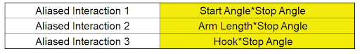
- Select Aliased Interactions using the drop-down list. Process knowledge, engineering or theory are used to make the selection and assume that the chosen interaction is dominant and the others are negligible. Aliased interactions are often associated with the largest main effects. Confirmation runs should always be used to validate the model. In this study, engineering knowledge was used to select all interactions that included the Stop Angle:
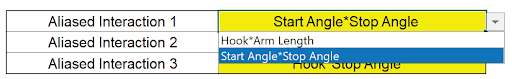
Tip: For Taguchi L8 Five to Six Factors and L16 Nine to Fourteen Factors, not all possible interactions are available in the drop-down list (they are aliased with main effects). If an interaction of interest is not available in any of the drop-down lists, please modify the Factor Names so that they are assigned to columns shown in the list and then select that interaction.
- A randomized run order was not given in the paper. The Outer Array Distance values are entered as shown:
Scroll to the right to view the calculated statistics:
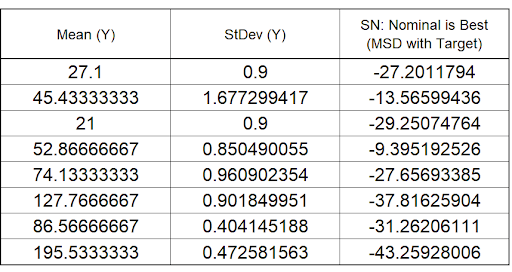
- We will focus our analysis on the Signal-To-Noise Ratio: Nominal is Best (MSD with Target). Since this design includes interactions, we will look at the Pareto of ANOVA SS (Sum-ofSquares) % Contribution for SN Ratios. Scroll right and down to view:
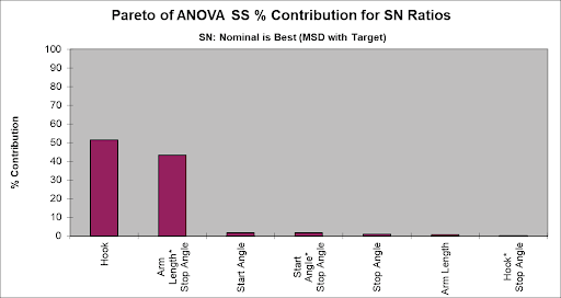
- We see that the Hook position and Arm Length* Stop Angle interaction are the dominant factors.
- Scroll down to view the Main Effects Plot for SN Ratios:
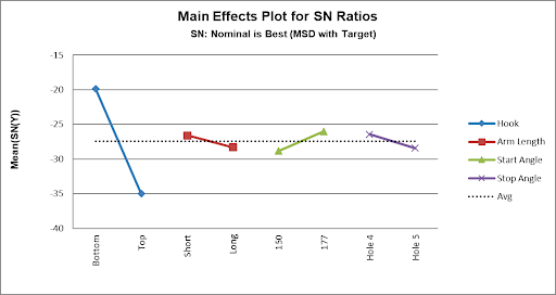
Setting Hook = Bottom and Start Angle = 177 maximizes the SN Ratio. (We will use the interaction plot to determine the optimum settings for Arm Length and Stop Angle).
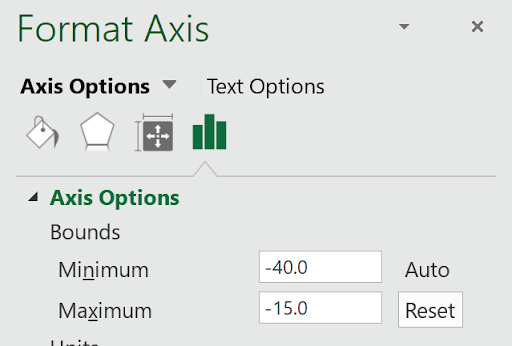
Note: The Y Axis has been adjusted to get a better scale (double click in the Y-Axis to open Excel Format Axis dialog, click Axis Options and set Maximum = -15 as shown).
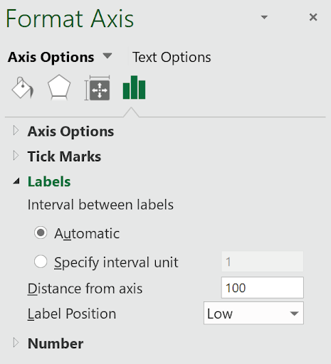
With the negative SN values, the default X-axis labels appear as on top. To change the X-Axis location to bottom, double click on the X-Axis to open Excel Format Axis dialog, click Axis Options, Labels and set Label Position to Low as shown)
- Scroll down to view the Interaction Plot for SN Ratios for the Arm Length * Stop Angle Interaction:
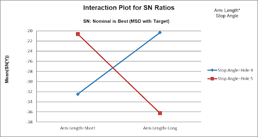
Here we can clearly see the large effect due to the two-way interaction. The effect that Arm Length has on Distance depends on what the Stop Angle is. The maximum SN Ratio is achieved with Arm Length = Long and Stop Angle = Hole 4.
Note 1: The Y-Axis has been adjusted to improve visibility (Maximum = -20).
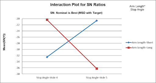
Note 2: The Interaction Plot X-axis/Legend factors may be switched by clicking on the chart, then select Excel Design > Switch Row/Column:

- From the above plots, we conclude that the optimum setting to produce a maximum SN Ratio for Distance = 50 is: Hook = Bottom, Arm Length = Long, Start Angle = 177 and Stop Angle = Hole 4.
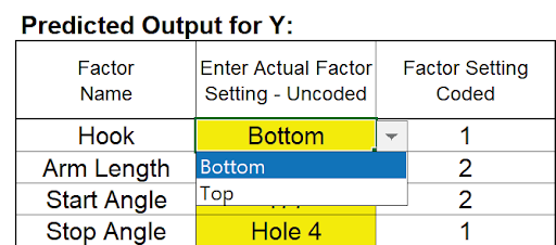
- Scroll up and left to enter these values in the Predicted Output Calculator. Factor settings can be selected from the drop-down list as shown:
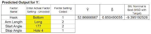
This gives the predicted Mean, Standard Deviation and SN Ratio for Distance and agrees with the results given in the paper. The predicted value of 52.9 inches is slightly off of the Target of 50 inches due to the discrete settings of the categorical factors.
Excel Solver cannot be used with this calculator to perform optimization, so we will use Multiple Regression and Solver, treating the Start Angle as continuous rather than categorical. This will allow interpolation in order to obtain a predicted Mean response of 50 inches
Multiple Regression and Excel Solver (Advanced Topics):
- The Taguchi L8 Orthogonal Array (or L8 Dummy Coding) may be analyzed using Multiple Regression Analysis, adding and removing terms from the model as necessary. However, for this example, we will not remove any terms from the model, following the analysis as performed in the paper.
- We will be analyzing the Mean Distance to refine the settings determined above from SN: Nominal is Best (MSD with Target).
- Highlight the L8 Orthogonal Array cells ( AM23:AW31) as shown.
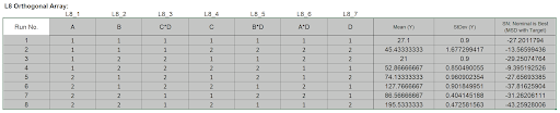
The Orthogonal Array displays the factor letters, not the names, so recall that A is Hook, B is Arm Length, C is Start Angle and D is Stop Angle.
- Click SigmaXL > Statistical Tools > Regression > Multiple Regression. Click Next.
- Select Mean (Y), click Numeric Response (Y) >>; now, one at a time carefully select the factors in the sequence: A, B, C, D, A*D, B*D and C*D, clicking Continuous Predictors (X) >> each time. Using this order will make subsequent analysis easier. Uncheck Display Residual Plots.
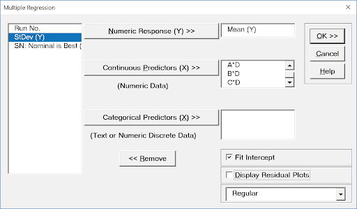
- Click OK. The resulting regression report is shown:
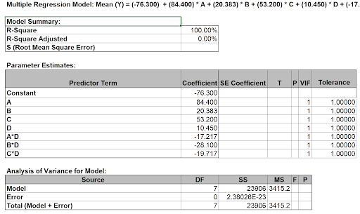
ANOVA and P-Values are not computed since there are no degrees of freedom for the error term.
- Now we will use the Predicted Response Calculator to determine the factor settings that achieve the Target value of 50 inches.
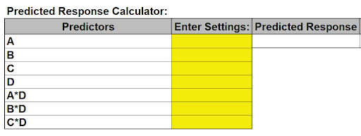
- All entries must be in coded units of 1 to 2 as given in the Orthogonal Array. While the calculator in the Taguchi Template uses strictly categorical factors, here we can use either categorical or continuous. We will use the categorical settings obtained from the SN Ratio analysis for: A = 1 (Hook = Bottom), B = 2 (Arm Length = Long), and D = 1 (Stop Angle = Hole 4). Factor C (Start Angle) is continuous and will be determined using Solver in order to achieve the Target Distance = 50 inches. The initial setting will be C = 2 (Start Angle = 177).
- Since the Taguchi Orthogonal Array is coded 1, 2 rather than -1, +1, we cannot simply multiply Factor A * Factor D to compute the A*D interaction.
- Turn on the Excel Row and Column headers in the Multiple Regression sheet: File > Options > Advanced. Scroll down to Display options for the worksheet. Check Show row and column headers. Click OK.
- In cell A*D (K16), enter the formula:
=1.5 - 2*(K12-1.5)*(K15-1.5)
This formula centers and scales the A (K12) and D (K15) values so that the A*D (K16) value will match the values in the Taguchi array.
- In cell B*D (K17) , enter the formula:
=1.5 - 2*(K13-1.5)*(K15-1.5)
- In cell C*D (K18), enter the formula:
=1.5 - 2*(K14-1.5)*(K15-1.5)
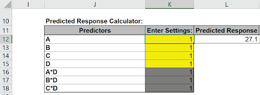
- Enter A = 1, B = 1, C =1, D=1 (be careful to not overwrite the formulas you may wish to change the K16 to K18 cell color as shown). The cells should show A*D = 1, B*D = 1 and C*D = 1.
Confidence and Prediction Intervals are not given because the model does not include an error term.
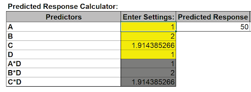
- As mentioned above, we will use the categorical settings obtained from the SN Ratio analysis, but Factor C (Start Angle) is continuous and will be determined using Solver in order to achieve the Target Distance = 50 inches. Enter the values as shown:
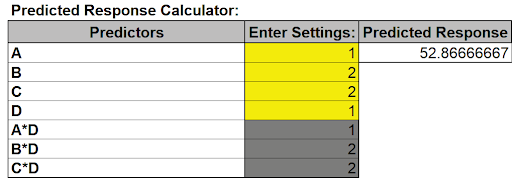
The initial Predicted Response matches the Mean in the Predicted Output given in the Taguchi Template
- Click Excel Data > Solver to open the Solver dialog (if the Solver menu option does not appear, click File > Options > Add-Ins. Adjacent to Manage Excel Add-ins, click Go. Check Solver Add-in. Click OK ). Set the Solver Parameters as shown:
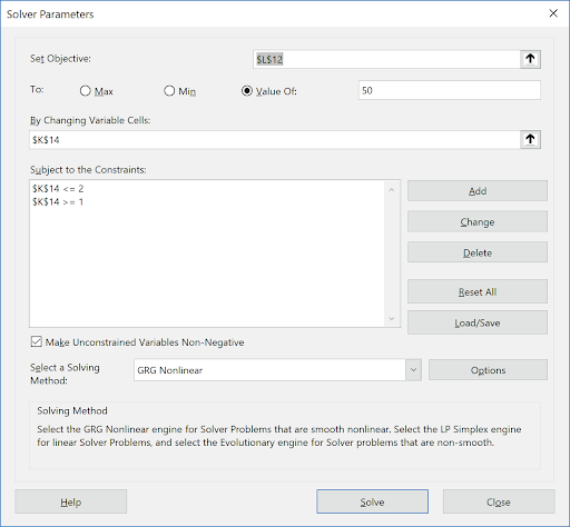
Cell L12 is the predicted response (Mean Distance). Solver will try to set this to the Target value of 50 inches. Cell K14 is the C Coded Factor Setting to be changed, with the constraint that the value is >=1 and <= 2. GRG Nonlinear is used here. (Note that if any of the Solver factors are modeled as categorical, Evolutionary is recommended).
- Click Solve.
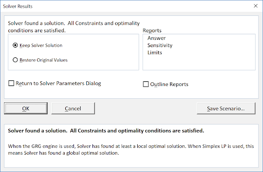
- The Predicted Response is 50 inches. Click OK to keep the Solver solution.
- Now we have to convert the coded C value to uncoded units. In cell L14, enter the formula:
=27*K14+123
This converts the coded 1 to 2 back to the uncoded 150 to 177 for the Start Angle.
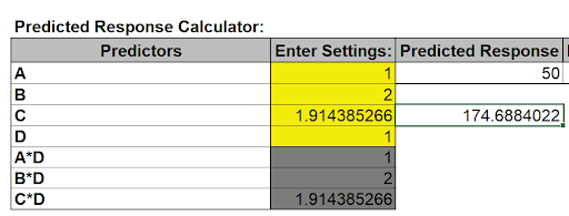
- The factor setting of 174.7 degrees to obtain a Mean Distance of 50 inches matches the value given in the paper. Confirmation runs were performed and validated the model prediction, resulting in greater precision than a theoretical model requiring 200 person-hours to develop!